
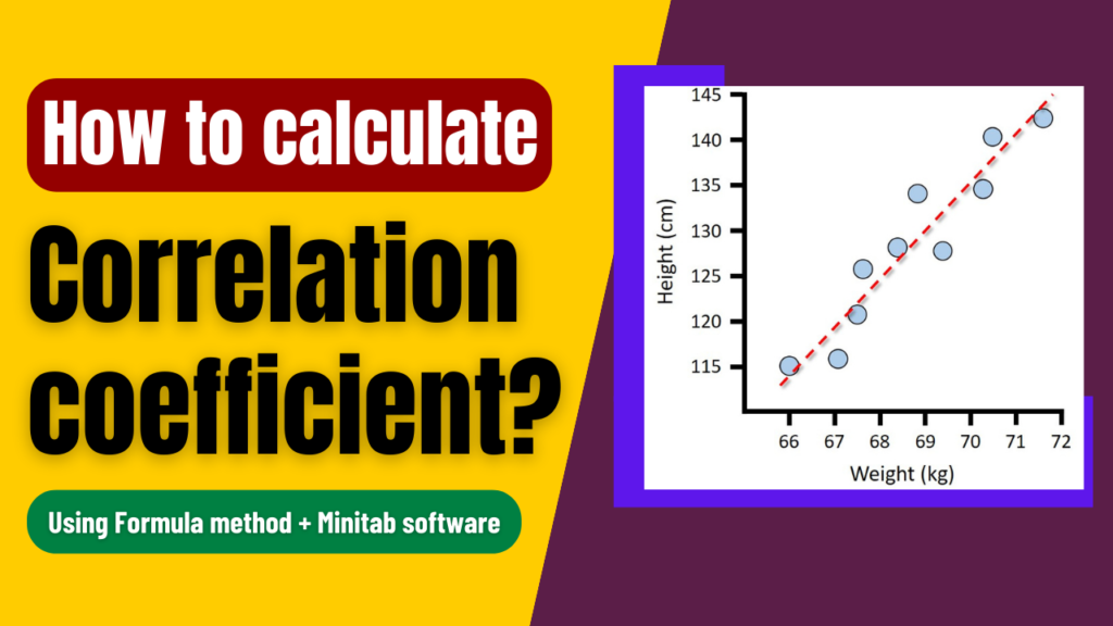
Have you ever wondered how to measure the strength of the relationship between two variables? You can use the Correlation coefficient, the best statistical measure that allows you to quantify the degree of association between two variables.
This powerful tool can help you measure the strength and direction of the relationship between two variables. You can calculate the correlation coefficient by hand using formulas as well as using software like Minitab and then interpret it.
In this article, we will understand the concept of correlation analysis, and types of correction, and then I will walk you through the steps to calculate the correlation coefficient by hand as well as using Minitab with the help of a practical example.
By the end of this article, you will be able to confidently analyze your data and interpret the correlation coefficient, and understand the relationship between your variables. So let’s get started…
What is correlation?
Correlation is a statistical measure that describes the strength and direction of the relationship between two variables with the help of a correlation coefficient. This tool helps researchers, data analysts understand how changes in one variable are related to changes in another variable.
It helps to determine whether two variables are related, and if so how strongly. This concept is essential in many fields, including psychology, economics, biology and sociology, business, process improvement, etc.
For example, in psychology researchers use correlation to examine the relationship between two variables, such as a person’s level of stress and their overall mental health.
In economics, correlation is used to understand how changes in one economic variable like interest rates are related to changes in another economic variable like the stock market.
In Lean Six Sigma, correlation is used to identify the relationship between process inputs and outputs. By analyzing the correlation between two variables, process improvement experts or lean six sigma practitioners can determine which input has a high impact on output.
By determining this they can focus their efforts on optimizing those inputs. Imagine a scenario where you are trying to improve the quality of the product. You have identified several potential factors that could affect product quality.
Such as raw materials, production methods, and machine settings. However, you are not sure which of these factors has the most significant impact on the quality of the product. This is where Correlation analysis comes in.
By collecting data on each of these variables and analyzing their relationships you can determine which factors are most strongly correlated with product quality.
Let’s say you might find that raw materials have a strong positive correlation with quality, while machine settings have a weak negative correlation. With this kind of data-based knowledge, you can make targeted improvements to the process.
Such as sourcing high-quality raw materials or adjusting machine settings to optimize performance. By focusing on the variables with the highest correlation to process outcomes you can achieve significant improvements in quality, efficiency, and customer satisfaction.
By understanding the relationships between process inputs and outputs, organizations can make data-driven decisions that lead to more efficient and effective processes. Let’s see 3 types of correlation as follows:
1. Positive correlation –
When two variables are positively correlated or you can say moving in the same direction. This means that as one variable increase, the other variable also increases.
For example – there is a positive correlation between the amount of exercise a person does and their level of physical fitness. The more exercise a person will do more he becomes physically fit.
2. Negative correlation –
When two variables are negatively correlated or you can say they are moving in opposite directions. This means that as one variable increases, the other variable decreases.
For example – There is a negative correlation between the amount of time a student spends watching TV and their academic performance. The more time student spends watching TV the lesser their academic performance will be.
3. Zero or No correlation –
When there is no relationship between two variables. This means that changes in one variable do not affect changes in another variable.
For example – There is no correlation between the color of a person’s look and their IQ. A person’s look does not have any positive or negative effect on their IQ level.
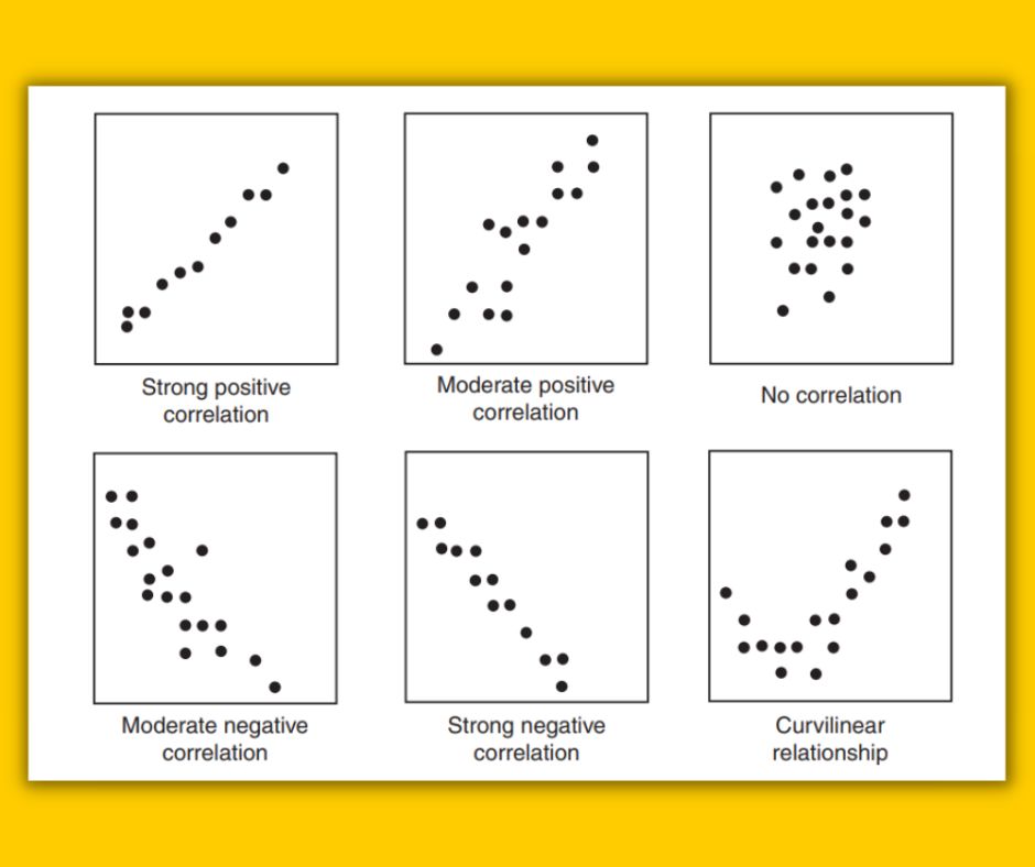
While doing correlation analysis practitioners generally use graphical tools called a scatter plot. A scatter plot graphically shows the relationship between two variables (positive, negative, zero) by analyzing the data for two variables.
You can see how correlation graphically looks for all 3 types of correlation. We will understand how to create a scatter plot using software later in this article –
- If there is a positive correlation, the data points will tend to cluster along a line sloping up and to the right.
- If there is a negative correlation, the data points will tend to cluster along a line sloping down and to the right.
- If there is no correlation, the points will be scattered randomly.
You can interpret the relationship between two variables using a scatter plot but if you can want to understand the exact strength of the correlation between two variables then you need to calculate the correlation coefficient.
This coefficient will tell you the strength of the correlation like whether there is a strong/weak positive correlation or there is strong/weak negative correlation.
With the help of mathematical value, you can easily understand the strength and degree of relationship between two variables. Now let’s understand the correlation coefficient in detail.
What is the correlation coefficient?
A correlation coefficient is a statistical measure that quantifies the strength and direction of the relationship between two variables. It is denoted by the symbol (r).
It is a fundamental tool used in statistics, data analysis, Lean Six Sigma, and machine learning to identify patterns in data and understand the association between two variables.
It is the number between -1 to +1, where the value of -1 indicates a perfect negative correlation, o indicates no correlation, and +1 indicates a perfect positive correlation.
It can be calculated using a formula that involves the covariances of two variables and their standard deviation. It can also be calculated using Minitab software. We will understand how to calculate it using both methods later in this article.
There are different types of correlation coefficients such as Pearson’s coefficient, Spearman’s coefficient, and Kendall’s coefficient, which are used depending on the type of data we have (Normal or Non-normal data).
Let’s understand them one by one –
Types of the correlation coefficient
There are several types of correlation coefficients that are commonly used in correlation analysis like Pearson’s correlation coefficient, Spearman’s rank correlation coefficient, and Kendall’s tau correlation coefficient.
These 3 are the most popular correlation coefficients used in different circumstances and can provide different insights into the relationship between variables. Let’s understand them one by one.
Pearson coefficient: (symbol ‘r’)
This coefficient measures the strength and direction of the linear relationship between two continuous variables (Variables like height, weight, time, etc). It basically measures how closely the relationship between two variables can be approximated by a straight line.
This coefficient ranges from -1 to +1. -1 indicates a perfect negative correlation in which when one variable goes up, the other goes down. + 1 indicates a perfect positive correlation in which when one variable goes up, the other also goes up).
Spearman’s rank coefficient: (symbol ‘ρ’)
This coefficient is used to assess the strength and direction of the non-linear and monotonic relationship between two continuous or ordinal variables (ordinal means variable which you can arrange in order form like automobile sizes, student ranks, etc)
Monotonic means the relationship is consistently increasing or decreasing but not necessarily at a constant rate. Instead of actual data, this coefficient is calculated by ranking the values of each variable and then comparing the ranks.
This coefficient also ranges from -1 to +1, where -1 indicates a perfect negative correlation and +1 indicates a perfect positive correlation.
Kendall’s rank coefficient: (symbol ‘τ’)
Kendall’s coefficient is another type of correlation coefficient that measures the non-linear relationship between two variables. It is similar to spearman’s coefficient but more robust to ties in data than spearman’s coefficient.
Similarly, this coefficient also ranges from -1 to +1, where -1 indicates a perfect negative correlation and +1 indicates a perfect positive correlation.
How to calculate the correlation coefficient?
We saw three different types of correlation coefficients out of which spearman’s and Kendall’s ranks are useful for non-linear relationships. But in the lean six sigma project, most of the time we have normal data with linear relationships.
So here I am going to discuss how to calculate the Pearson coefficient because it is useful for linear relationships. For this article, my focus is on Pearson coefficient calculation. Right!
There are two ways we can calculate the Pearson correlation coefficient i.e. manually by using formulas, using software like Minitab. I am going to calculate that using these methods with the help of one practical example.
Example – Buy used car case study example
We have the data about the age of the car and the mileage of each car (i.e. how many km each car drove). Here we want to understand how the age of the car correlates with the mileage of the car.
Here the X variable is the age of the car and the Y variable is the total km driven. Both are continuous variables and we have to find out whether these two variables are in a positive linear relationship or negative. See the data below.
| Sr.No | Age of car in years (X variable) | Total Kms driven (Y variable) |
| 1 | 1.2 | 25 |
| 2 | 5.3 | 75 |
| 3 | 4.6 | 92 |
| 4 | 0.7 | 13 |
| 5 | 2.1 | 110 |
| 6 | 2.5 | 64 |
| 7 | 1.9 | 29 |
| 8 | 4.3 | 105 |
| 9 | 6.4 | 233 |
| 10 | 3.8 | 126 |
| 11 | 2.2 | 57 |
| 12 | 5.4 | 115 |
To calculate the correlation coefficient between these 2 variables we are going to use the manual as well as a software method. Let’s calculate it and interpret the final results.
Calculate by hand using the formula
In this method, we are going to calculate the correlation coefficient using the standard formula. We will do all the calculations in the table itself and then put all the values directly into the formula to get the final ‘r’ value.
The Pearson correlation coefficient formula standard formula:

Where, n – Total quantity of variable
∑X – Total of the first variable (Age of car in yrs)
∑Y – Total of the second variable (Total KM driven)
∑XY – Total sum of the product of the first and second variable
∑X² – Sum of the square of the first value
∑Y² – Sum of the square of the second value
Example data with all calculations:
| Sr.No | Age of car in years ( X variable) | Total Kms driven ( Y variable) | XY | X² | Y² |
| 1 | 1.2 | 25 | 30.0 | 1.44 | 625 |
| 2 | 5.3 | 75 | 397.5 | 28.09 | 5625 |
| 3 | 4.6 | 92 | 423.2 | 21.16 | 8464 |
| 4 | 0.7 | 13 | 9.1 | 0.49 | 169 |
| 5 | 2.1 | 110 | 231 | 4.41 | 12100 |
| 6 | 2.5 | 64 | 160 | 6.25 | 4096 |
| 7 | 1.9 | 29 | 55.1 | 3.61 | 841 |
| 8 | 4.3 | 105 | 451.5 | 18.49 | 11025 |
| 9 | 6.4 | 233 | 1491.2 | 40.96 | 54289 |
| 10 | 3.8 | 126 | 478.8 | 14.44 | 15876 |
| 11 | 2.2 | 57 | 125.4 | 4.84 | 3249 |
| 12 | 5.4 | 115 | 621 | 29.16 | 13225 |
| Total | 40.4 | 1044 | 4473.8 | 173.34 | 129584 |
We created 3 extra columns i.e. XY, X², Y², and calculated respective values for each X and Y variable. These three column values you need, to calculate the final correlation coefficient (‘r’).
For first X = 1.2 and Y = 25, the XY = 1.2 × 25 = 30, X² = 1.2 × 1.2 = 1.44, Y² = 25 × 25 = 625. That’s how you need to calculate XY, X², and Y² for each row data value.
After that calculate the total sum for each column and put all these values in the formula:
n = 12, ∑X = 40.4, ∑Y = 1044, ∑XY = 4473.8, ∑X² = 173.34, ∑Y² = 129584
r = 12 (4473.8) – (40.4)(1044) / √ [ 12 (173.34) – (40.4)²] [ 12 (129584) – (1044)²]
r = 53685.6 – 42,177.6 / √ [ 2080.08 – 1632.16] [ 1555008 – 1089936]
r = 11508 / √ [ 447.92 ] [465072]
r = 11508 / √ 208315050.24
r = 11508 / 14433.1233
r = 0.79 = 0.80
By the manual calculation method, we got Pearson correlation coefficient = 0.8 for this example. We will interpret this value later, let’s first calculate ‘r’ using Minitab.
Calculate using Minitab
Let’s calculate the correlation coefficient for the same example using Minitab and follow the step-by-step procedure.
Step-1: Select data > select Stat option from the menu > Basic statistics > Correlation
First, you need to Load your data in Minitab, in this example, we have 2 column table with two variables i.e. age of the car and the mileage of the car. Insert the data values for both variables in the Minitab worksheet.
After that select data and select the ‘Stat’ option from the main menu (you can see that on top) and then click on Basic Statistics and in that select ‘correlation’.

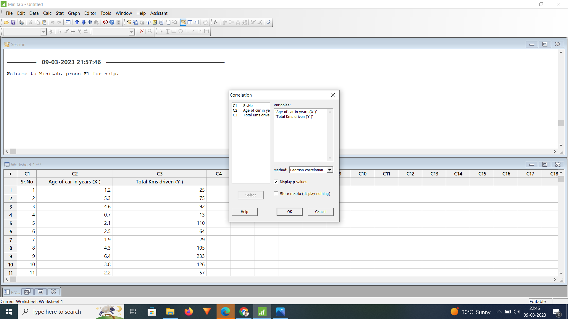
Step-2: Click on Correlation > Select variables (X & Y) > Select coefficient type > Click ‘Ok’
The moment you click on the correlation, a new dialogue box appears on the Minitab worksheet. In that box, select the column (variables)that contains data you want to analyze i.e. age of the car and total km driven.
You can do this by clicking on the column names in the list on the left and then clicking the arrow button to move them to the list on the right.
After that you can see the method option in the dialogue box, there you need to select the type of correlation coefficient you want to calculate.
The default option is Pearson’s correlation coefficient so keep that as it is. Below that click the display p-value box and at last click ‘ok’ after confirming that all the things you selected are accurate.
Step-3: Click ‘OK’ to run the analysis > See the results in the Minitab window
Click ok on the dialogue box to run the analysis and then results will appear in the Minitab output window. You can see the correlation coefficient value along with the p-value. (Check out – What is P-value)
You can see the final result that, here also got the correlation coefficient value = 0.797 = 0.80. Hence By using Minitab, we got Pearson correlation coefficient = 0.8 for this example.

Step-4: Visually, you can see the correlation using a scatter plot
Follow these Simple steps to create a scatter plot and visually interpret the relationship between two variables.
- Main menu > Graph > Scatter plot – See (1) image
- Select simple from the dialogue box > Click ok – See (2) image
- New dialogue box open > Select Y and X variable in the box > Click ok – See (3) image
- Scatter plot ready in the window – See (4) image
This scatter plot visually shows that there is a linear positive relationship between two variables. With the increase in the age of cars, there is an increase in total km driven (direct proportion). (Check out – Correlation coefficient calculator)

Interpretation of correlation coefficient
We calculated the correlation coefficient using the formula method as well as using Minitab software. In both cases, we got the coefficient value r = 0.80.
As we know the correlation coefficient (r) range is -1 to +1 which indicates that +1 means strong positive correlation, -1 means strong negative correlation and 0 means no correlation.
In our example, the r is 0.80 which is close to the +1 and it concludes that there is a pretty good positive correlation between the age of cars and total km driven.
With an increase in the age of cars, there is an increase in total km driven. You can say that it is a near to strong positive relationship between these two variables.
Limitations of the correlation coefficient
- It only measures the linear relationship between two variables. It may not capture the non-linear relationship, which can be present in some data.
- It does not imply causation. Just because two variables are correlated doesn’t mean one variable has an impact on the other. There may be some other variables that are influencing the relationships.
- The presence of outliers in data can greatly affect the value of the correlation coefficient. Outlier makes it difficult to interpret the strength of the relationship between two variables.
- It only measures the strength and direction of the relationship between two variables. It does not provide information about the magnitude of the effect, for magnitude, you need to go for regression analysis.
- It can be affected by the range and distribution of the data. For example, if the range of one variable is much larger than another variable, then the correlation coefficient may be biased towards the variable with a larger range.
Conclusion
Calculating the correlation coefficient is important for data analysis and understanding the relationship between variables. Throughout the article, we have learned the two methods to calculate the coefficient value i.e. formula method and Minitab software.
The formula method involves some arithmetic calculations and is easy to use for small datasets. On the other hand, Minitab software can help you calculate the correlation coefficient quickly and accurately irrespective of the size of the datasets.
Regardless of the method you choose, calculating r is important to quantify the relationship between two variables. With the help of the r value, you can make informed decisions about variables and draw a more accurate conclusion from your data.
If you found this article useful then please share it in your network and subscribe to get more such articles every week.

I found the article very impressive and thought-provoking.
Thanks for your feedback!