

Six Sigma methodology makes an improvement with the help of data. But to make this improvement happen, we need to derive Six Sigma Metrics (like DPU, DPMO, PPM, RTY) from the data because these metrics help businesses to make a decision about the processes.
These Metrics are nothing but the system or standard of measurement. These metrics capture the knowledge which then translated into opportunities for improvement and growth. In this article, we will understand the important Six Sigma metrics with the help of a practical example. So let’s start…..
Types of six sigma metrics –
In any process improvement endeavor the ultimate objectives are to make the process Better, Faster, and Cheaper, to do this Lean Six Sigma Metrics plays an important role. If you make the process better by eliminating defects you will make it faster. If You choose to make a process faster, you will have to eliminate defects to be as fast as you can be.
Similarly, if you make the process better and faster, you will necessarily make it cheaper. So, all the Six Sigma metrics fall under three categories given below:
- To make the process better – Defects per unit, Defects per million opportunities, rolled throughput yield, etc.
- To make the process faster – Cycle time
- To make the process cheaper – Cost of poor quality
Before we get into the depth of six sigma metrics, let’s understand the two types of six sigma metrics.
The Primary Six Sigma metrics –
This metric is a very important measure in the six sigma project, this metric is a quantified measure of the defect or primary issue of the project and it serves as the indicator of project success.
It has some important characteristics that we need to understand. Examples of the primary metrics are customer satisfaction, on-time delivery to customers, cost-effective products, quality of the product, etc.
- There is only one primary metric per project.
- It should be linked to the primary business measure or we can say aligned to business objectives.
- It should be easily measurable and can be expressed with an equation.
- It should be tied to the problem statement.
The Secondary Six Sigma metrics –
Secondary metrics are put in place to measure potential changes that may occur as a result of making changes to our primary metric and they will measure positive and negative consequences as a result of changes in the process.
Per project, we can have multiple secondary metrics. Examples of secondary metrics are cycle time, lead time, rework hours, etc. As per equation Y = f(x), if Y is the primary metric then X is the secondary metric.
Primary and secondary metrics should be continually measured and frequently updated like daily, weekly, monthly, etc during the project’s lifecycle. These metrics should be expressed pictorially over time with a run chart or time series plot.
It is very important that you should be aware of these two important metrics. Now turn our attention toward important six sigma metrics and try to understand them with examples.
Here, we are going to understand the 1st category metrics like DPU, DPMO, and RTY with the help of an example. Let’s use an example of stamped and anodized aluminum L-bracket with four 4 step processes: material testing, treatment(anodizing), dimension (stamping process), and properties verification.
Refer to the information given in the below chart to calculate metrics.
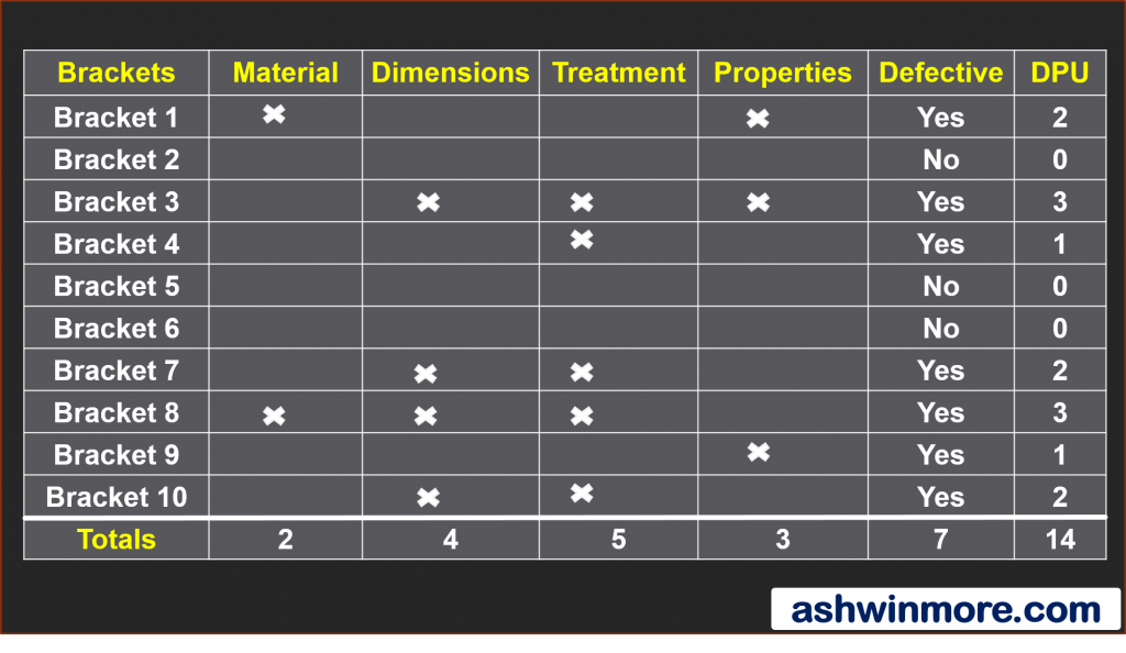
This chart shows the data for 10 L-brackets, which are tested under four processes like material testing, stamping process, anodizing treatment, and properties verification. The cross mark indicates that a particular bracket shows defects under a different process.
Eg- let’s say bracket-1, shows a cross mark in the material testing and properties verification process which means bracket-1 shows one defect each in these two processes, and overall it is considered as a defective bracket.
Similarly, if you look at bracket-2 it doesn’t show any defect under four processes because there is no cross mark hence bracket-2 is considered as the non-defective bracket. After that in the last two columns defects per unit, values are given for each bracket.
And which bracket is defective (Yes/no) that information is also given. The last row of “Total” indicates how many brackets failed in each process. Now use this information to calculate six sigma metrics.
Read more – What is Six Sigma methodology?
1. Defects per unit: (DPU) –
Defects per Unit (DPU) quantifies individual defects on a unit or you can say DPU is the number of defects per manufactured unit and calculating DPU is one of the ways to identify how well a process performs.
Now look at the above chart, there are a total of 10 brackets (units) produced out of which 7 are defective and the total no of defects are 14 in all brackets.
Almost all the brackets have multiple defects, it is important that you need to know the concept of “Defects” and “Defectives” before calculating DPU. “defect” means a physical count of all errors on a unit, and “defectives” means a unit with two or more defects.
Eg-
DPU = Total defects / Total units produced
= 14 / 10 = 1.4
So there are 1.4 defects per unit in this process.
2. Defects per million opportunities: (DPMO)
Before calculating DPMO let’s first understand the concept of “defects per opportunity”, DPO describes the average defects in each unit produced or you can say it is a measure of the probability of defects.
Now look at the above chart, we have a total of 10 units and total defects are equal to 14 also every unit or bracket is tested through 4 processes.
So it may possible that that bracket shows defects during each process hence we can say that there are maximum of 4 defect opportunities for each bracket.
As defect opportunities are 4 for each unit and we have a total of 10 units that means total defect opportunities are 10*4 = 40.
By using these values we can easily calculate the DPO value… Defect opportunities per unit = 4 Total defects opportunities = 10 * 4 = 40
Defects per opportunity = Total defects / Total defects opportunity
= 14 / 40 = 0.35
Hence average defects in each unit produced = 0.35 DPO
Then comes Defects per million opportunities (DPMO), which is also a probability measure. It calculates the “probability that a given process will produce X defect opportunities per million units produced”.
Here we are considering a constant number of 1 million and finding out how many defects opportunities are there in 1 million units. To calculate it just multiply DPO by 1 million. (10^6).
DPMO = DPO * 1000000 = 0.35 * 1000000 = 350,000
Hence there are 350,000 Defects opportunities in 1 million units.
3. Parts per million: (PPM)
PPM defective is one of the simplest metrics to understand. It is used to count the number of defective parts per million parts produced or we can say it refers to the expected number of parts out of 1 million that you can expect to be defective.
DPMO and PPM are different from each other, DPMO is a measure of “Defects” and it provides insight about defects opportunities per part in the process.
While PPM is a measure of “Defectives” it does not provide insight about defects opportunity per part because to calculate PPM we consider the Defective unit as a whole. It is a popular measure when dealing with proportion defectives, where a large number of units are involved in the process.
Now take a look at our chart, the 2nd last column shows how many defective brackets are there so out of 10 brackets there are 7 defectives means all 7 brackets show at least one defect in any of the four processes.
( Bracket no -1, 3,4, 7,8,9,10 defective brackets).
In this example, 7 defective units out of 10 means defectives percentage of a population are equal to 7 / 10 = 0.7
PPM = Defectives percentages of a population * 1000000
= 0.7 * 1000000 = 700,000
Hence 7 defectives out of 10 units yield a PPM of 700,000 i.e 700,000 defectives in 1 million units.
4. First pass yield: (FPY)
The first pass yield is a metric used to determine how a process is performing in relation to the number of good units. It is simply the number of good units (defect-free) produced divided by the number of total units going into the process.
The standard formula is as follows-
FPY = Total defect-free units / Total units entered in the process
For process 1 – (material verification process) There are 2 failures in 10 units means only 8 units are defect-free at the first time hence FPY = 8 / 10 = 0.80
For process 2 – (stamping process) There are 4 failures in 10 units means only 6 units are defect-free at the first time hence FPY = 6 / 10 = 0.60
For process 3 – (anodizing process) There are 5 failures in 10 units means only 5 units are defect-free at the first time hence FPY = 5 / 10 = 0.50
For process 4 – (properties verification process) There are 3 failures in 10 units means only 7 units are defect-free at the first time hence FPY = 7 / 10 = 0.70
5. Rolled throughput yield: (RTY)
Rolled throughput yield is considered one of the most appropriate metrics for problem-solving. It is the probability that a process with more than one step will produce defect-free units.
To calculate RTY we need to first calculate the yield for each process step and then by multiplying the yield of each process step, we will get our RTY of the complete process.
RTY = FPY1 * FPY2 * FPY3 * FPY4
We have already calculated First pass yield values for each step of the process. FPY1 = 0.80, FPY2 = 0.60, FPY3 = 0.50, FPY4 = 0.70 now just put these values in the above formulae and calculate the final RTY.
RTY = 0.80 * 0.60 * 0.50 * 0.70 = 0.168 = 16.8%
As RTY = 16.8%, only 16.8 % of brackets (units) were accepted in the entire process, and 83.2% (100-16.8) of brackets were rejected due to defects hence we can say that the process is performing very badly because, in every 10 brackets, only 1.68 = 2 brackets are defect-free while all the remaining are defectives.
Read more – What is Rolled throughput yield? RTY vs FTY
6. Sigma level of the process:
To better understand the sigma level, you need to know the DPMO numbers and corresponding sigma values. From the table a DPMO of 691,462 equates to 1 sigma, DPMO of 66,807 equates to 3 sigma.
Similarly, a DPMO of 233 equates to 5sigma, and a DPMO of 3.4 equates to 6sigma. The Six Sigma method measures the capability of a process using the ‘sigma level’. The aim is to achieve a sigma level of at least six, which equates to less than 3.4 DPMO.
Now, coming back to our example, we calculated the DPMO for this aluminum bracket example and we got the value of DPMO = 350,000. so if you look at the six sigma table you will find that 350,000 lies between DPMO of 308,537 and 691,462.
This means the sigma level is between 1 and 2 but as 350,000 is closer to 308,537, we can conclude that this process is operating at the 2 sigma level. If you want to learn practically how to calculate all these six sigma metrics then join us – EALSS Lean Six Sigma training program.
So definitely this process needs lots of improvement to achieve 6 sigma level performance. That’s how we can find the sigma level of any process. Check out the sigma level calculator.

Get certified in Lean Six Sigma – EALSS Academy
Conclusion –
These are some of the important Six Sigma metrics commonly used in six sigma projects. I discussed DPO, DPMO, PPM, RTY, FTY, and Sigma levels of the process using an aluminum bracket example and also discussed how to calculate these metrics with the help of mathematical formulae.
I hope you got the clarity about Six Sigma metrics and how to calculate them with this article. If you found this article useful then please share this in your network and subscribe to get more such articles.


I just like the valuable info you supply on your articles.
I’ll bookmark your blog and check again here frequently.
I’m relatively certain I’ll be informed many new stuff proper here!
Best of luck for the following!
Thanks for your feedback
I’ve been surfing online more than 2 hours today, yet I never found any interesting article like yours.
It is pretty worth enough for me. In my opinion, if all web owners and bloggers made good content as you did, the net will be much more useful
than ever before.
Thanks for your feedback
I scouted many referals and material on 6 sigma. none of them are as informative as yours. I wish to learn more on y=fx hope it’s in line in future training.
Thanks for making us learn
Thanks for the feedback and please subscribe to get more such content for free.
Simple and powerful, thank you.
Your welcome!
In part 2 – The last sentence should say ‘there are 350,000 defects per million opportunities’.
There are 4,000,000 defect opportunities in 1 million units (1,000,000 x 4).
I enjoy reading your articles!
Thanks for your feedback!